Combining Chronos2 with PyMC-Marketing for marketing forecasting
Your marketing team just allocated $30 million for next quarter’s campaigns. The strategy depends on predicted economic conditions, seasonal patterns, unemployment, and competitive dynamics. There’s one problem: the employment rates and weather patterns your model needs don’t exist yet. How do you input them?
This is the scenario planning paradox that keeps data scientists up at night. Marketing Mix Models are good at untangling causal relationships – they tell you how each dollar spent on TV versus digital affects sales while accounting for external factors. But when it comes to planning future campaigns, these models hit a wall: they need control variables that haven’t happened yet.
What if you could combine the causal clarity of MMMs with modern time series forecasting to project into the future with quantifiable confidence?
Two parallel advances
We’re at an interesting intersection of two developments, both driven by recent computational gains, that are changing how predictive analytics works in practice.
On one side, there’s the Bayesian MMM renaissance. Probabilistic programming frameworks like PyMC have made Bayesian MMMs practical at scale. What used to require weeks of custom MCMC implementation now fits into readable code, with sampling algorithms like NUTS making inference feasible even for high-dimensional, hierarchically structured problems across markets.
On the other, there’s the foundational model wave in forecasting. The same transformer architectures that reshaped NLP are now being applied to time series. Models like Chronos2, released by Amazon in 2025, are pre-trained on large corpora of time series data and achieve strong accuracy out of the box, without domain-specific tuning. They capture complex temporal patterns through attention mechanisms that would have been computationally prohibitive just a few years ago.
Both advances share a common enabler: dramatically more compute and better algorithms. A hierarchical Bayesian MMM that might have taken days to converge in 2018 now runs in hours on JAX-backed samplers. Training and deploying transformer-based time series models has become practical for everyday business use.
The architecture of hybrid prediction
The appeal of combining these approaches is that their strengths are complementary. MMMs encode explicit causal structure. They know that advertising drives sales through specific mechanisms like adstock (how effects linger over time) and saturation (how channels become less effective at high spend). Foundational models, on the other hand, excel at pure pattern recognition, learning seasonalities and trends from data without needing structural assumptions.
Here’s how I put these together in practice:
# Step 1: Train MMM on historical data to learn causal relationships
mmm = MMM(
    channel_columns=["tv_spend", "search_spend"],
    control_columns=["avg_employment", "avg_temp"],
    adstock=GeometricAdstock(l_max=13),
    saturation=LogisticSaturation(),
)
mmm.fit(X_historical, y_historical)

# Step 2: Use Chronos2 to forecast future control variables
pipeline = Chronos2Pipeline.from_pretrained(
    "amazon/chronos-t5-base",
    device_map="auto",
    torch_dtype=torch.bfloat16,
)
control_forecasts = pipeline.predict(
    context=historical_controls,
    prediction_length=52,  # weeks ahead
)

# Step 3: Combine forecasts with planned media spend for predictions
X_future = combine_media_plan_with_forecasted_controls(
    media_plan, control_forecasts
)
sales_predictions = mmm.predict(X_future)
Each model does what it’s best at. The MMM keeps its causal interpretation – you still know exactly how much each marketing dollar contributes to sales. The foundational model handles the messy job of forecasting external factors without requiring you to build separate models for employment, weather, and every other control.
A realistic testing ground
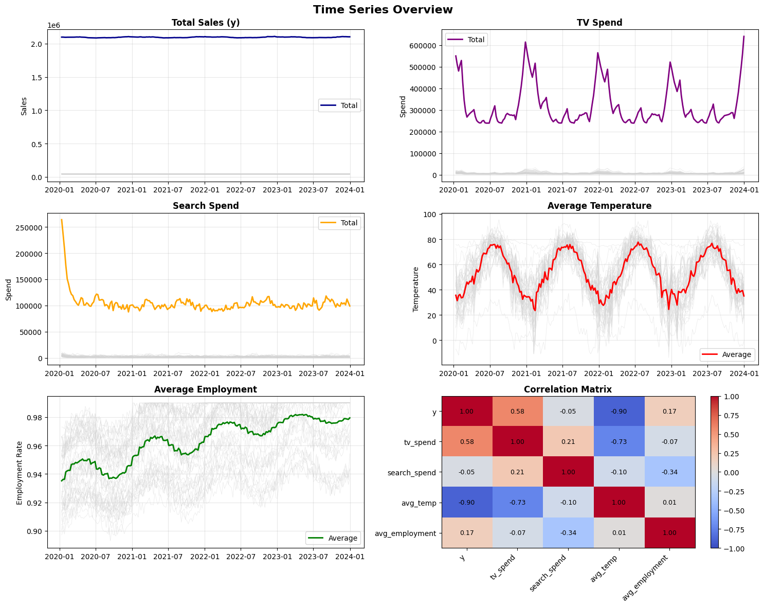
To test this approach, I built a hierarchical dataset that mirrors real-world complexity. The sales figures are simulated using known MMM dynamics, but the control variables (temperature and employment rates) come from actual U.S. historical data across 50 states over four years (2020–2023). Media spend patterns and effect sizes are calibrated to match typical CPG marketing scenarios, with TV spending ranging from $10,000 to $20,000 weekly per state and search spend between $2,000 and $8,000.
This gives 10,400 observations (50 states times 208 weeks) with realistic seasonality, geographic variation, and the kinds of correlations you’d encounter in production. Because I know the ground truth, I can rigorously evaluate how forecast uncertainty propagates through the causal model.
Quantifying the cascade of uncertainty
The interesting question isn’t whether this works, but how much forecast errors in control variables affect final sales predictions. I trained the MMM on three years of data (2020–2022) and reserved 2023 for evaluation. This mirrors a real scenario planning exercise where you’re using historical relationships to project into an uncertain future.
First, how well does Chronos2 forecast the control variables?
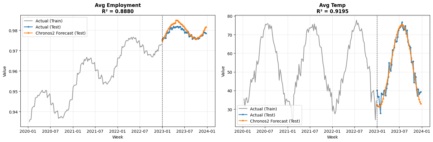
The forecasts track actual patterns well. They pick up seasonal cycles in temperature and gradual trends in employment. But how does this translate to MMM prediction accuracy?
The math of error propagation
To understand how control forecast errors affect MMM predictions, it helps to look at the mathematical relationship. The core idea is straightforward: errors in control variables propagate to your sales predictions in proportion to how much those controls matter to your model.
In our MMM, each prediction combines two components:
\[\hat{y} = m + \gamma^{\top} x\]
Here, \(m\) is the contribution from media channels (TV, search, etc.), while \(\gamma^{\top} x\) captures the influence of control variables like employment rates and temperature. The vector \(\gamma\) contains coefficients that quantify how much each control affects sales, and \(x\) contains the control values.
When we forecast into the future, we replace the true controls \(x\) with our Chronos2 predictions \(\hat{x}\). This introduces an error:
\[\Delta \hat{y} = \gamma^{\top} (\hat{x} - x)\]
Think of it as a multiplication effect: if a control variable has a large coefficient (it matters a lot to sales) AND you forecast it poorly, the error gets amplified. But even large forecast errors in unimportant controls barely move the final prediction.
This leads to a practical bound. The additional MAPE from using forecasted controls is bounded by:
\[\mathbb{E}[|\Delta \text{MAPE}|] \leq \sum_{j=1}^{p} w_j \cdot \text{MAPE}_j\]
where \(\text{MAPE}_j\) is the forecast accuracy for control \(j\) and \(w_j = \mathbb{E}[|\gamma_j| \cdot |x_j|/|y|]\) is its relative importance, the fraction of sales variation this control explains.
The practitioner’s rule: Control MAPE x Control Share = Added MMM MAPE
For example, if temperature and employment together explain 30% of your sales variation, and you forecast them with 10% MAPE, expect roughly 3% additional error in your sales predictions. This quick multiplication tells you whether your control forecasts are good enough for reliable planning.
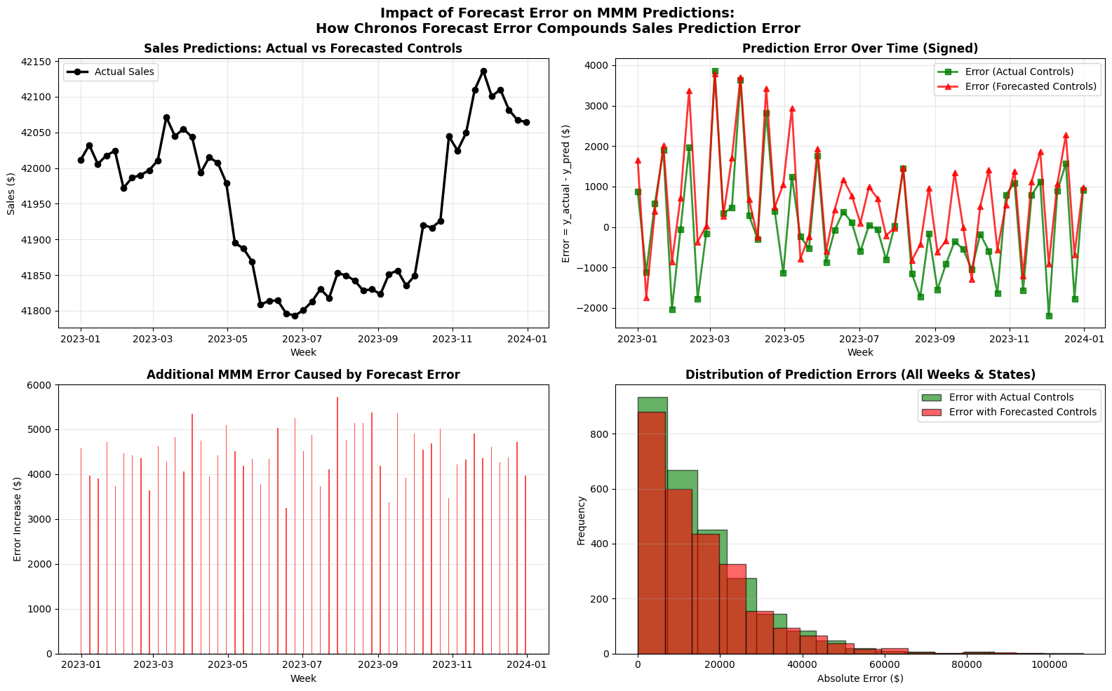
The empirical results match the math:
- With actual controls: MAPE of 2.89%, RMSE of $1,517
- With forecasted controls: MAPE of 3.23%, RMSE of $1,642
- Degradation: only +0.34% MAPE increase, despite 52-week-ahead forecasts
Why is the degradation so small? In this dataset, control variables (temperature and employment) explain roughly 15% of sales variation. Chronos2 forecasts these controls with about 3% MAPE on average. Applying the rule: 15% x 3% = 0.45% expected MAPE increase. The actual increase was 0.34%, even better than the conservative estimate.
This small degradation makes intuitive sense. Even with the uncertainty of long-range forecasts, final predictions stay accurate because the controls, while meaningful, don’t dominate sales dynamics. Media spend remains the primary driver.
Putting it into production
Running this in production requires some thought around engineering. Here’s what has worked well.
Model training cadence. Retrain the MMM monthly or quarterly as new data arrives. Update control forecasts weekly for rolling planning horizons.
Uncertainty quantification. Don’t settle for point forecasts. Generate prediction intervals for controls and propagate them through the MMM:
# Generate multiple forecast samples
control_samples = pipeline.predict(
    context=historical,
    num_samples=100,
    quantile_levels=[0.1, 0.5, 0.9]
)

# Propagate through MMM for uncertainty bounds
predictions_with_uncertainty = []
for sample in control_samples:
    pred = mmm.predict(combine_with_media(media_plan, sample))
    predictions_with_uncertainty.append(pred)
Monitoring and validation. Track these metrics in production: control forecast accuracy (MAPE by variable), MMM prediction error on recent holdout data, divergence between planned and actual media spend, and posterior predictive checks for MMM assumptions.
Where this approach fits best
This hybrid architecture works well in specific situations.
Quarterly planning cycles, where you need to allocate budgets 3–6 months ahead based on expected market conditions.
Geographic expansion, where you’re entering new markets with historical control data but no sales history. Train the MMM on existing markets and use Chronos2 forecasts for the new region.
Scenario analysis, where you generate multiple control scenarios (optimistic/pessimistic economic conditions) and see how optimal media allocation changes under each.
What comes next
Combining Bayesian MMMs with foundational time series models opens up forward-looking scenario planning that traditional MMMs can’t do on their own. The causal structure stays intact, the forecasting handles the parts you don’t know yet, and the math gives you a clear picture of how much uncertainty you’re adding.
That said, I want to be honest about where this is still early. The error propagation bounds I’ve shown here assume relatively well-behaved control variables. In practice, structural breaks (a pandemic, a policy change, a competitor entering the market) can throw off even good forecasting models. The Chronos2 forecasts are strong for variables with clear seasonal or trend patterns, but less predictable controls will naturally introduce more error. You should always validate the approach on your own data before making big budget decisions based on it.
The tools are all open source. PyMC-Marketing handles the MMM side, and Chronos2 is available through HuggingFace Transformers with pre-trained weights ready for inference. A good starting point is the MMM quickstart guide and then layering in the Chronos2 forecasting pipeline for your control variables.
This analysis used PyMC-Marketing v0.9.0 and Chronos2 pre-trained models. The complete code, including data generation and evaluation scripts, is available on GitHub.