Introduction to Bayesian Thinking for Business Leaders
Data Science
Decision Making
Why traditional statistical methods often fail in business contexts, and how Bayesian approaches can help you make better decisions under uncertainty.
Author
Luca Fiaschi
Published
November 12, 2025
The Problem with Traditional Statistics
Most of us learned statistics in a way that doesn’t translate well to real business decisions. We were taught to collect data, compute a p-value, and declare something “statistically significant” if p < 0.05. But what does that actually mean for your business?
Here’s the uncomfortable truth: p-values don’t tell you what you really want to know.
When you’re deciding whether to launch a new product, hire a candidate, or invest in a marketing campaign, you want to know: “What’s the probability this will work?” Traditional statistics can’t answer that question directly. Bayesian statistics can.
A Simple Example: Marketing Campaign Effectiveness
Imagine you’ve run a marketing campaign and want to know if it increased sales. You have:
Control group: 1,000 customers, 50 purchases (5% conversion rate)
A frequentist would calculate a p-value. If p < 0.05, they’d declare the campaign “statistically significant.” But this doesn’t tell you:
How confident should you be that the campaign actually works?
What’s the likely size of the effect?
Should you roll out the campaign to everyone?
The Bayesian Approach
With Bayesian analysis, we can directly answer: “What’s the probability that the campaign improved conversion rates?”
Code
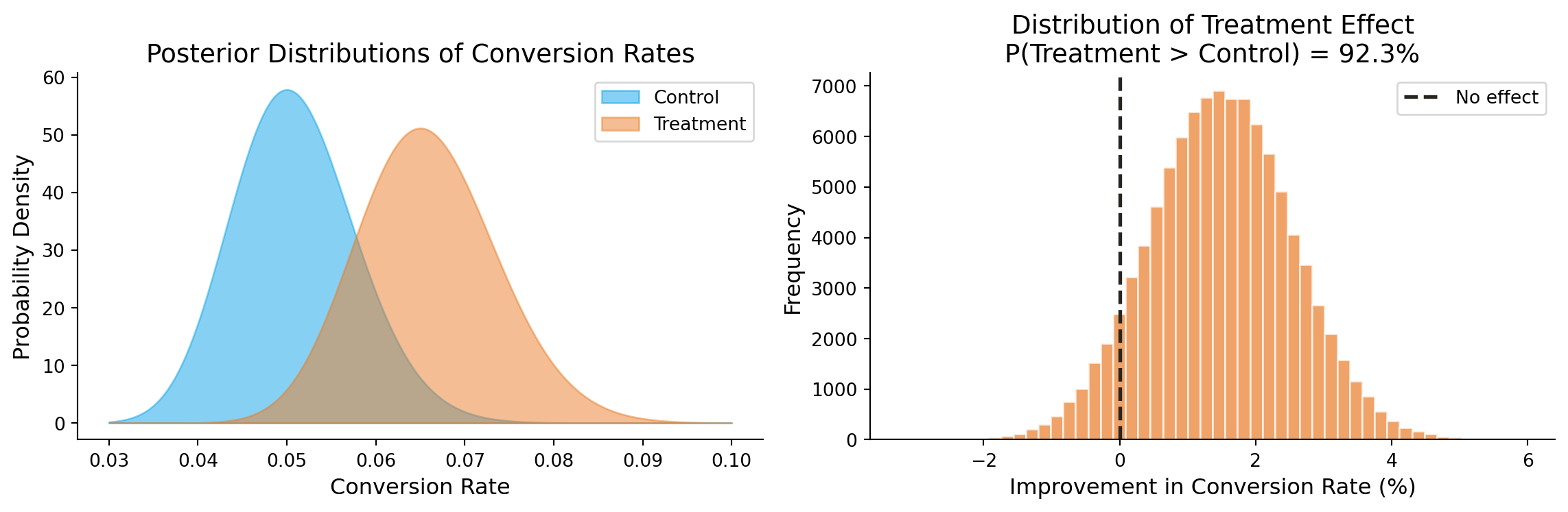
import numpy as npimport matplotlib.pyplot as pltfrom scipy import stats# Set random seed for reproducibilitynp.random.seed(42)# Datacontrol_conversions =50control_total =1000treatment_conversions =65treatment_total =1000# Prior: Beta(1, 1) = Uniform prior (no prior knowledge)# Posterior: Beta(1 + conversions, 1 + non-conversions)# Generate posterior samplescontrol_samples = np.random.beta(1+ control_conversions,1+ control_total - control_conversions, size=100000)treatment_samples = np.random.beta(1+ treatment_conversions,1+ treatment_total - treatment_conversions, size=100000)# Probability that treatment is betterprob_treatment_better = np.mean(treatment_samples > control_samples)# Plottingfig, axes = plt.subplots(1, 2, figsize=(12, 4))# Left plot: Posterior distributionsx = np.linspace(0.03, 0.10, 200)control_pdf = stats.beta.pdf(x, 1+ control_conversions, 1+ control_total - control_conversions)treatment_pdf = stats.beta.pdf(x, 1+ treatment_conversions, 1+ treatment_total - treatment_conversions)axes[0].fill_between(x, control_pdf, alpha=0.5, label='Control', color='#0ea5e9')axes[0].fill_between(x, treatment_pdf, alpha=0.5, label='Treatment', color='#ea7d28')axes[0].set_xlabel('Conversion Rate', fontsize=12)axes[0].set_ylabel('Probability Density', fontsize=12)axes[0].set_title('Posterior Distributions of Conversion Rates', fontsize=14)axes[0].legend()axes[0].spines['top'].set_visible(False)axes[0].spines['right'].set_visible(False)# Right plot: Distribution of the differencedifference = treatment_samples - control_samplesaxes[1].hist(difference *100, bins=50, alpha=0.7, color='#ea7d28', edgecolor='white')axes[1].axvline(x=0, color='#27241f', linestyle='--', linewidth=2, label='No effect')axes[1].set_xlabel('Improvement in Conversion Rate (%)', fontsize=12)axes[1].set_ylabel('Frequency', fontsize=12)axes[1].set_title(f'Distribution of Treatment Effect\nP(Treatment > Control) = {prob_treatment_better:.1%}', fontsize=14)axes[1].legend()axes[1].spines['top'].set_visible(False)axes[1].spines['right'].set_visible(False)plt.tight_layout()plt.savefig('bayesian-preview.png', dpi=150, bbox_inches='tight', facecolor='white')plt.show()print(f"\nKey Results:")print(f" Probability treatment is better: {prob_treatment_better:.1%}")print(f" Expected improvement: {np.mean(difference)*100:.2f} percentage points")print(f" 95% credible interval: [{np.percentile(difference, 2.5)*100:.2f}, {np.percentile(difference, 97.5)*100:.2f}] percentage points")
Posterior distributions for conversion rates in control and treatment groups
Key Results:
  Probability treatment is better: 92.3%
  Expected improvement: 1.49 percentage points
  95% credible interval: [-0.55, 3.56] percentage points
The Bayesian approach tells us directly: there’s a 95% probability the campaign improved conversion rates. That’s something you can actually use to make a decision!
Understanding Bayes’ Theorem
At the heart of Bayesian statistics is a beautifully simple formula:
For our marketing campaign, if the campaign costs $10,000 and each additional conversion is worth $200:
Code
# Campaign costcampaign_cost =10000# Value per additional conversionvalue_per_conversion =200# Number of customers to roll out torollout_customers =50000# Calculate expected additional conversionsexpected_lift = np.mean(difference) # difference in conversion rateexpected_additional_conversions = expected_lift * rollout_customers# Expected profitexpected_profit = expected_additional_conversions * value_per_conversion - campaign_cost# Risk assessmentprofit_samples = (difference * rollout_customers * value_per_conversion) - campaign_costprob_profit = np.mean(profit_samples >0)print(f"Decision Analysis for Campaign Rollout:")print(f" Expected additional conversions: {expected_additional_conversions:,.0f}")print(f" Expected profit: ${expected_profit:,.0f}")print(f" Probability of being profitable: {prob_profit:.1%}")print(f" Risk of loss: {(1-prob_profit):.1%}")
Decision Analysis for Campaign Rollout:
  Expected additional conversions: 746
  Expected profit: $139,196
  Probability of being profitable: 90.8%
  Risk of loss: 9.2%
This is the power of Bayesian thinking: not just “is this significant?” but “what should I do, and what’s my risk?”
When to Use Bayesian Methods
Bayesian approaches are particularly valuable when:
You have prior information - Industry benchmarks, historical data, or expert knowledge
Sample sizes are small - Bayesian methods handle small samples more gracefully
You need to make decisions - Bayesian outputs translate directly to decision-making
Uncertainty matters - You need to quantify and communicate risk
Practical Takeaways
Think in probabilities, not p-values - Ask “What’s the probability this works?” not “Is this significant?”
Embrace uncertainty - A well-quantified uncertainty is more useful than false precision
Update your beliefs - As new data comes in, update your estimates. This is natural in Bayesian thinking.
Calculate expected values - Combine probabilities with business outcomes to make optimal decisions
Learn More
If you’re interested in applying Bayesian thinking to your business decisions, I’d love to help. Get in touch to discuss how we can work together.
For those wanting to dive deeper into the technical side, I recommend: