How to build a brand measurement system: a Bayesian playbook

Marketing Science

Brand

Bayesian Methods

An opinionated playbook for data science leaders: connect brand tracking, Bayesian MMM, experiments, and VARX to commercial decisions.

Author

Luca Fiaschi

Published

September 15, 2026

What observing Away taught me about measurement

At Rocket Internet, I watched one of its investments, Away Travel (Away), build a suitcase brand people knew. I understood that brand mattered. I did not yet have a credible way to measure what its activity added to demand later.

Away gave people reasons to talk about a suitcase through product design, travel stories, press coverage, partnerships, and the customer experience. The harder question was commercial: how much later demand did that work create, relative to what would have happened anyway?

One execution makes the problem concrete. Away paid to amplify Vogue’s launch coverage on Facebook. The click took the reader to Vogue, not to a product page.

Away's Facebook post anchors a diagram showing its click going to Vogue editorial coverage, engagement creating visible attention, and a later route through consideration, direct visits or branded search, and the Away store to purchase. — Figure 1: Away’s Facebook post sent readers to Vogue’s editorial coverage. Attention to that story could later contribute to a direct visit or branded search, but the screenshot does not establish incremental sales. Original screenshot and campaign account: Away case study.

A buyer could encounter the story, remember the company, and search for Away when they need luggage. Search appears close to the sale; the earlier influence does not.

The published launch case (an excellent write-up by my former boss, Enrico Ferrari) describes activity that can amplify a brand’s value. It leaves the central measurement problem open: connecting that activity to the demand and revenue that follow.

I get this question repeatedly in consulting engagements. The practical question is whether brand activity created enough later contribution to justify its full cost. The approach below separates immediate response from slower demand and tests the uncertain links before turning either into a spending decision.

Why the measurement choice changes the growth strategy

The measurement choice changes the budget. If search gets credit for customers who first encountered the brand elsewhere, search looks like the sensible place to move money. A short-term MMM can reinforce that choice when its response window misses earlier activity’s slower effects. The company then cuts work that helped create demand while continuing to reach people already ready to buy.

Reported acquisition efficiency can improve for a while. Without enough new demand, however, the next customer becomes more expensive and growth is harder to sustain. Effective brand activity can make more buyers familiar with the company before they need the product, give them a reason to choose it, and support the price they will pay.

Buyers first remember and evaluate the company. Someone shopping for luggage may recall Away before comparing alternatives. That is mental availability: coming to mind in a buying situation rather than simply recognizing a logo. Credibility can make an offer worth considering and reduce price sensitivity, as research on brand choice and price sensitivity suggests. Design and associations can give someone a reason to prefer the product beyond its functional specifications.

The commercial effect may arrive months after the advertising: a customer remembers the brand now, chooses it when the need arises, and may buy again later. Brand measurement therefore follows consideration, realized prices, and repeat purchase—not just a survey score. Keller’s customer-based brand equity poses the useful question: how does knowing the brand change a buyer’s response? The system must follow that response far enough to see the commercial consequence.

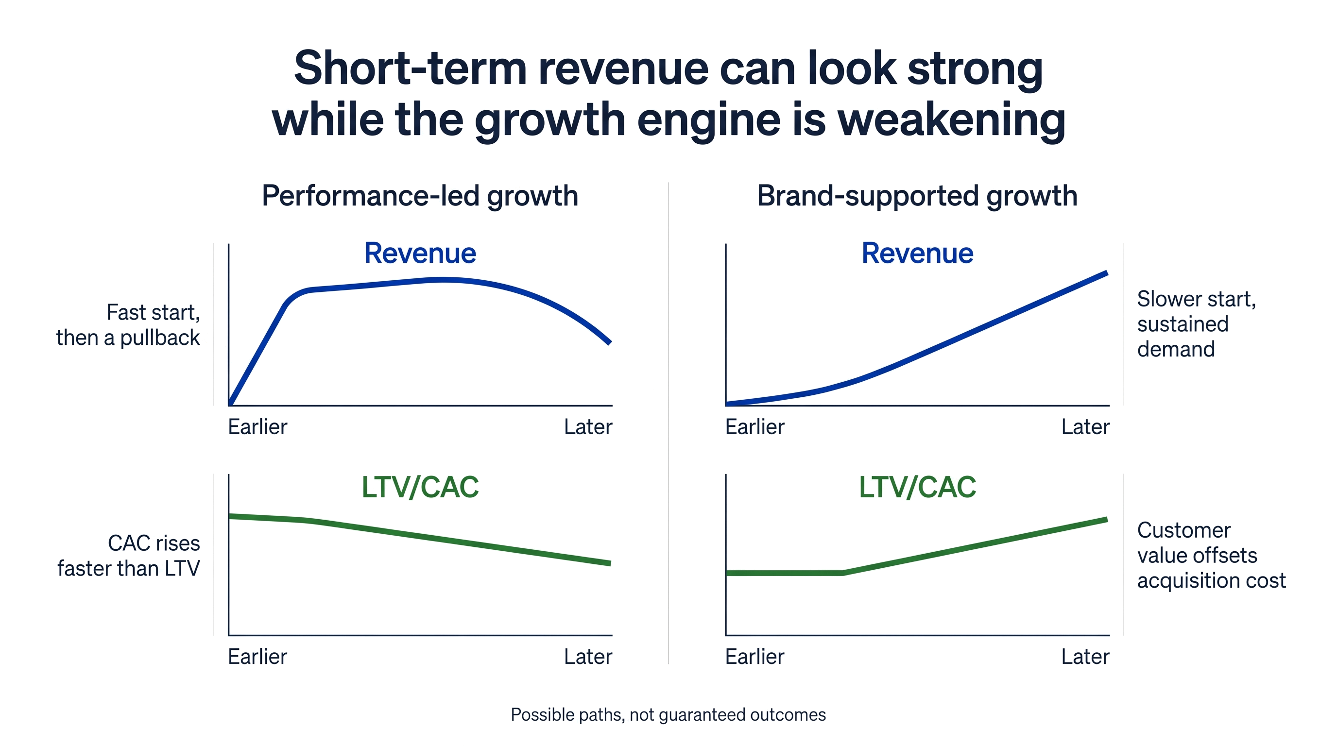
Figure 2: The figure sketches how growth can stall as acquisition gets more expensive, while stronger demand or customer contribution can keep it going.

The decision is whether those effects occur in this business, how long they take, and whether their value covers the investment.

Why isn’t a media mix model enough?

A media mix model is a useful starting point: it estimates how sales respond to media spending while accounting for seasonality and other commercial influences. The budget decision also depends on whether advertising changes later demand through familiarity, consideration, or willingness to pay. A direct spending-to-sales model cannot distinguish those pathways on its own.

The first issue is timing. Geometric adstock gives a single exposure its largest weight immediately, then reduces that weight by the same proportion each week. That can discount a campaign before a potential buyer needs the product.

With weekly retention $\alpha$, the weight after $h$ weeks relative to its initial weight is:

\[ \frac{w_h}{w_0} = \alpha^h \]

At 70% weekly retention, only 1.0% of the initial weight remains after 13 weeks. If $\alpha = 0.8$, the model retains 80% each week and loses 20%, leaving 5.5% after 13 weeks. Even retaining 90% each week leaves only 25.4%: almost three quarters has decayed away. A large fraction retained from one week to the next does not mean a large fraction survives a quarter.

Figure 3: Geometric-adstock weights after one exposure, relative to week zero. At week 13, retention rates of 0.70, 0.80, and 0.90 leave 1.0%, 5.5%, and 25.4%, respectively. These are decay weights, not measured brand or sales effects; no finite lag cutoff is applied.

Geometric adstock is useful for direct response, but it cannot establish a brand pathway. Under 80% retention, the model gives an exposure from 13 weeks ago about one eighteenth of an exposure today; an eight-week lag cutoff assigns it no weight at all.

Delayed and other flexible adstock functions can change the response shape. They still do not tell us whether a slower sales response came through consideration, distribution, or something else. That is why the system adds tracker measures, models their relationship to later demand, and uses experiments where the budget depends on a causal claim.

The system I would build

Build the system in three moves. Stage 1 uses a Bayesian MMM to separate immediate media response from a flexible sales baseline. Stage 2 models that baseline alongside brand tracking and organic demand. Experiments test the uncertain links that would change the spending decision.

Peter Cain’s purchase-journey framework connects brand measures to evolving base sales. I adapt that idea using a Bayesian MMM and a vector autoregression with external drivers (VARX), which models several time series together. Ryan O’Sullivan’s walkthrough explores this approach to long-term brand measurement.

I use this architecture when a company has usable sales and media histories but its immediate-response model may miss slower demand. Starting with two stages makes the system easier to fit, diagnose, and revise than a single joint model.

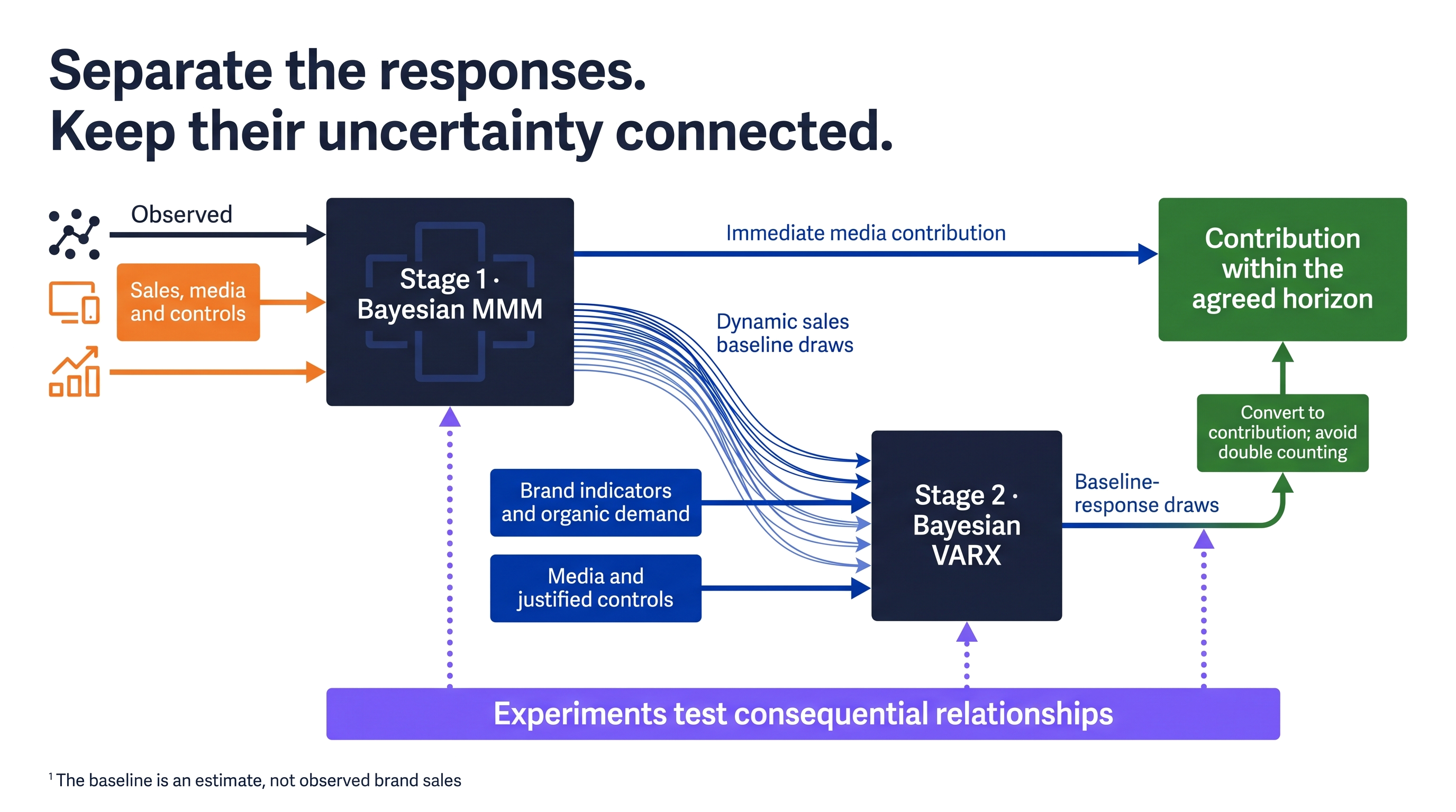
Figure 4: Stage 1 passes plausible dynamic sales baseline trajectories into Stage 2. Immediate media contribution remains separate. Experiments inform both stages, and the responses are combined in contribution dollars without counting the same modeled response twice.

Stage 1 separates immediate media contribution, seasonality, and justified controls from a time-varying intercept. I call that intercept the dynamic sales baseline: the changing sales level left after those modeled components are separated.

Stage 2 makes that Stage 1 baseline its sales target and models it with selected brand indicators and organic demand in a Bayesian VARX. Each series uses its own history and earlier values of the other series; media enters as a driver. The model returns week-by-week responses to a specified spending change. Because the baseline is a residual sales component rather than observed brand value, interpret it alongside controls, business changes, and experimental evidence.

Immediate media contribution stays in Stage 1; Stage 2 estimates response only within the separate baseline component. Before combining them, the analyst must check that the Stage 2 target excludes Stage 1’s immediate media term, keep each contribution on its own component path, and convert both to contribution dollars. Adding a Stage 2 estimate of total sales to Stage 1 media contribution would otherwise count some response twice.

Sparse or unstable tracking calls for a narrower experiment or commercial analysis first.

Before fitting, finance and the budget owner agree on full campaign cost, the contribution measure, the payback period, and the decision threshold. Those choices define the output the model must deliver.

The implementation sequence

Work through the eight phases below and return to the data whenever a diagnostic changes the decision.

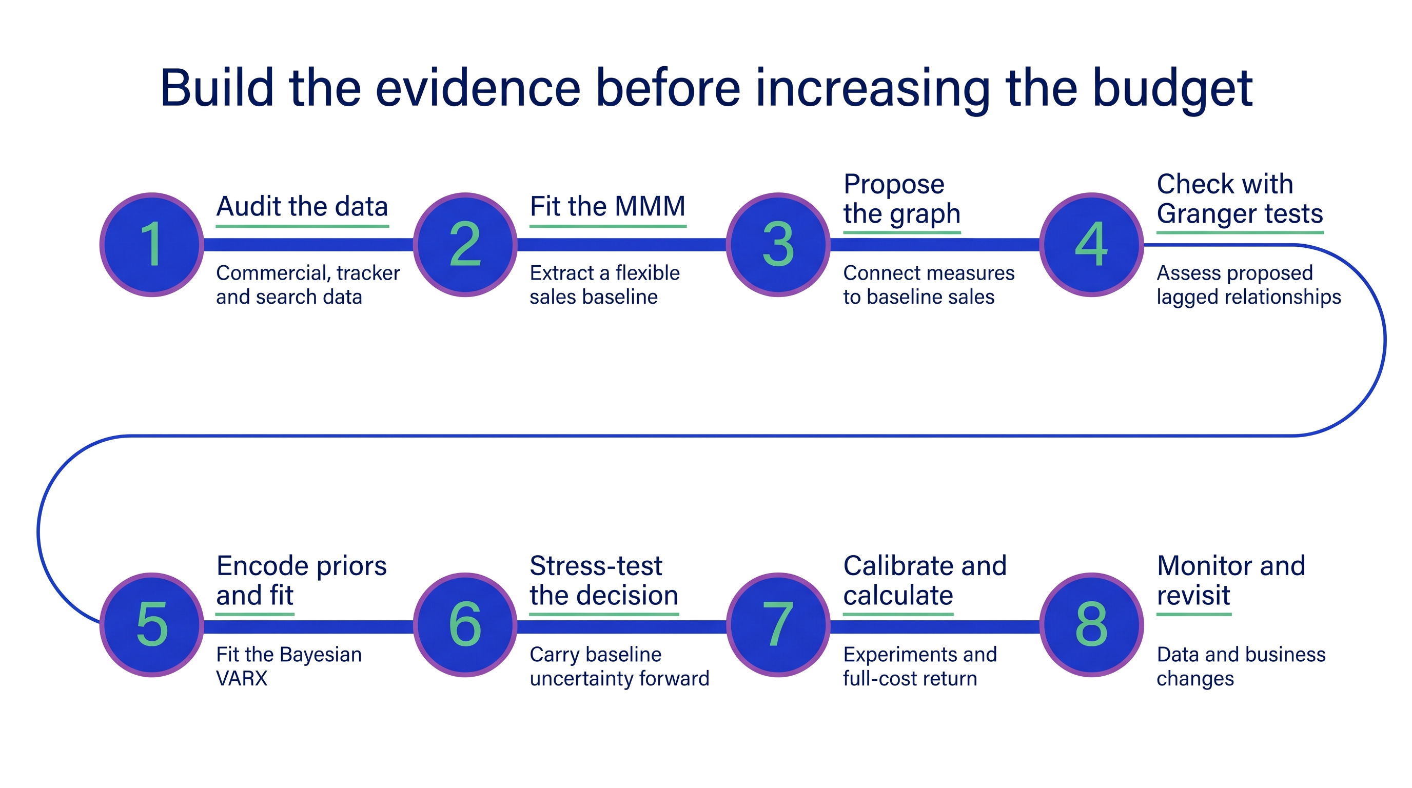
Figure 5: Eight implementation phases: audit the data, fit the MMM, propose the graph, check with Granger tests, encode priors and fit the VARX, stress-test, calibrate and calculate, and monitor.

Each phase leaves an inspectable handoff, from data definitions to the calculation that converts response into contribution.

1. Audit and complete the measurement data

Start by listing the evidence that can test the brand hypothesis.

The first inputs are familiar from a conventional MMM or CRM analysis: commercial outcomes, media activity, and customer behavior. The additions are brand tracking and organic-demand signals such as branded search, Share of Search, and organic traffic. Those measures are less common in a standard MMM, but they help test the pathway from brand activity to later sales.

Put every series on one calendar. Record its owner, definition, refresh cadence, and known breaks, then plot the raw histories before fitting. Start with a small set of commercial and brand measures that could plausibly affect sales; a perfect data warehouse can wait.

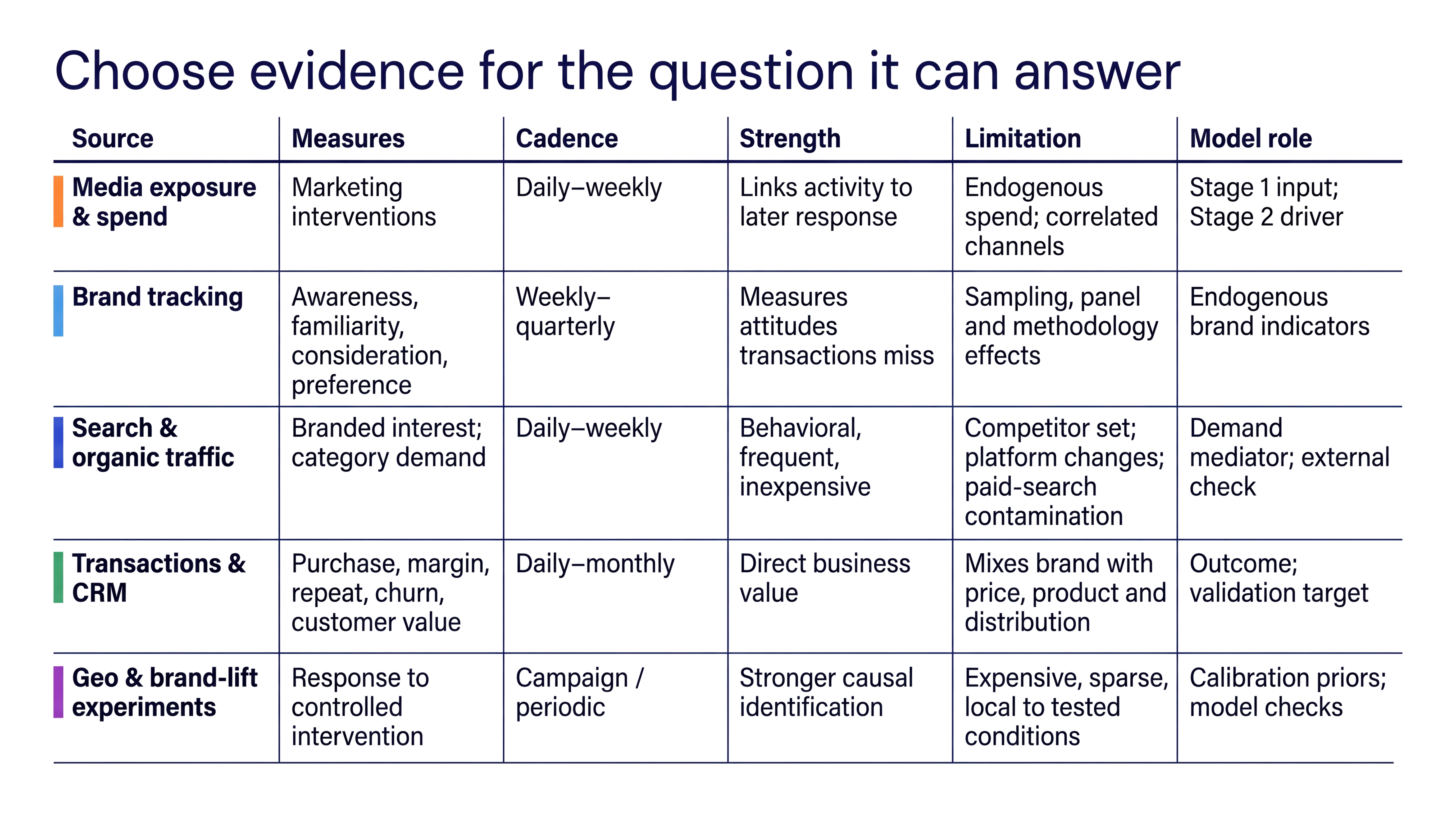
The inventory below separates the evidence sources by what they can contribute.

Swipe horizontally to read the full figure.

Figure 6: Five evidence sources with their measures, cadence, strengths, limitations, and model roles. The table is a data inventory, not a proven causal sequence.

Obtain brand-tracking data deliberately

Brand tracking is usually a repeated cross-sectional survey: the same core questionnaire is fielded to a comparable target population at a regular cadence. Keep the target definition, sampling quotas, wording, scales, and fieldwork method stable. A broad consumer tracker often starts with roughly 300–400 completed interviews per market per wave.

Turn a small set of survey answers into time series. Ask unaided awareness (“Which luggage brands come to mind?”), aided awareness, consideration, and one or two questions tied to the hypothesis, such as whether the brand feels distinctive or worth paying more for. Teams can buy this through a self-serve platform such as Attest, a subscription tracker such as YouGov BrandIndex, or a custom provider such as Latana or Kantar. Choose based on the required questionnaire, competitor coverage, and sampling; public Latana entry pricing starts at €7,900 per market per year for awareness tracking.

2. Fit the short-term MMM and extract the flexible baseline

Stage 1 has one job: use a standard PyMC-Marketing MMM to separate immediate media, seasonal, and known-control contributions from a sales baseline that can change over time. That baseline becomes the Stage 2 sales target.

Use a time-varying intercept for that baseline. In PyMC-Marketing, a Hilbert-space Gaussian-process approximation gives the team a smooth but flexible curve for sales movement outside channels, seasonality, and controls. Tune it so it neither forces gradual sales movement into media nor absorbs a channel response without evidence.

The PyMC-Marketing brand-effects notebook provides an implementation reference. This schematic uses the current API and makes the Gaussian-process baseline explicit; the HSGP prior must be chosen for the time scale of the business rather than copied unchanged.

Schematic Stage 1 implementation

from pymc_marketing.hsgp_kwargs import HSGPKwargs
from pymc_marketing.mmm import MMM, GeometricAdstock, LogisticSaturation

# A flexible, time-varying sales baseline.
baseline_hsgp = HSGPKwargs(
    m=50,
    L=None,
    eta_lam=1.0,
    ls_mu=8.0,
    ls_sigma=4.0,
)

mmm = MMM(
    date_column="date_week",
    channel_columns=channel_columns,
    control_columns=control_columns,
    adstock=GeometricAdstock(l_max=8),
    saturation=LogisticSaturation(),
    yearly_seasonality=10,
    time_varying_intercept=True,
    model_config={"intercept_tvp_config": baseline_hsgp},
)

mmm.build_model(X, y)
mmm.sample_prior_predictive(X, y, samples=1_000)
idata = mmm.fit(
    X=X,
    y=y,
    chains=4,
    draws=1_000,
    tune=1_000,
    target_accept=0.95,
)

baseline_draws = idata.posterior["intercept_contribution_original_scale"]

Run prior predictive checks before fitting. Then inspect posterior predictions, convergence diagnostics, residual autocorrelation, and rolling or holdout performance.

Stage 2 takes the Stage 1 baseline as its sales target and models it alongside selected brand-tracking measures and organic demand. The uncertainty handoff happens in Phase 6, where Stage 2 is refit across a sample of plausible Stage 1 baselines.

3. Choose the data that could explain the sales baseline

The VARX models how the Stage 1 sales baseline changes over time, using its own history and earlier movements in other measured variables. It also models how those variables respond to one another and to media spending. The question is whether changes in buyer attitudes and active interest help explain the sales movement left by the MMM.

Return to the data collected in Phase 1. Survey-based awareness measures whether buyers know the brand; consideration measures whether they would consider buying it. Branded organic search records active interest. These are useful candidates because a buyer may become familiar with Away, consider it later, and search when they need luggage. The model estimates whether earlier movements in these measures predict later baseline sales.

Build a time-aligned dataset with the Stage 1 baseline, the selected tracker measures, search, and spend. The baseline, awareness, consideration, and search become the outcomes modeled together. Media spend enters as a supplied driver, along with relevant commercial controls. Each outcome is predicted from its own past values, past values of the other outcomes, and the drivers. Use the sampling frequency supported by the tracker; repeating a monthly survey value across weekly rows does not create weekly observations.

Draw the candidate graph from these measured series. Each arrow should express a hypothesis and a plausible response time. For example, does greater consideration precede more branded search, and does that search precede higher baseline sales?

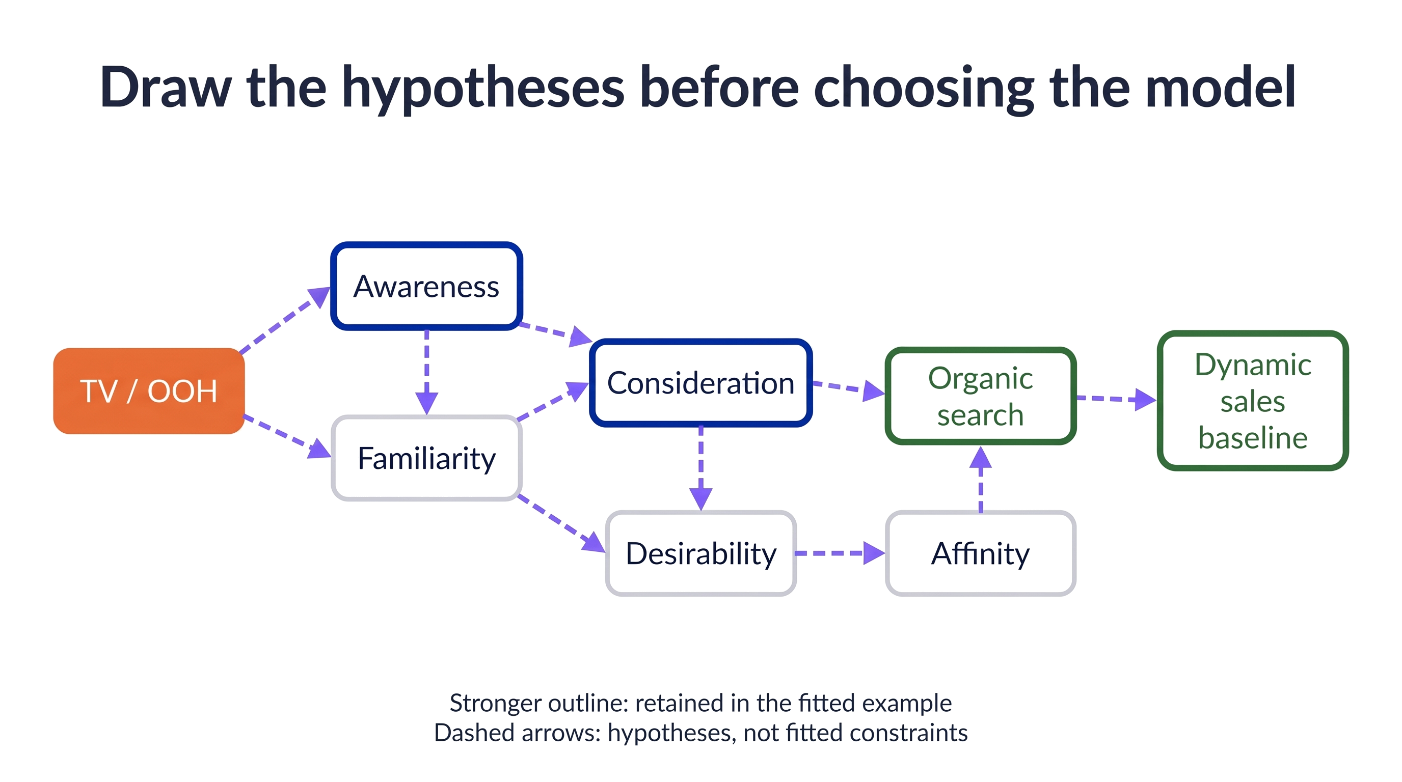
Figure 7: A candidate hypothesis map. The numerical illustration retains awareness, consideration, organic search, and the dynamic sales baseline. The arrows are proposed mechanisms, not discovered causal facts or hard-zero constraints on the fitted coefficients.

The graph separates outcomes from external drivers. Putting spend outside the outcome vector does not make it statistically exogenous: budget owners respond to forecasts, inventory, and recent performance, so spending can share shocks with sales.

Document those common causes and feedback decisions. An intervention interpretation needs an identification argument that addresses them, or experimental variation. The graph makes the gaps visible.

4. Check the proposed relationships with Granger tests

Use conventional Granger causality tests as another check on the candidate graph. For a proposed consideration-to-search edge, ask whether past consideration improves prediction of search after including search’s own history and the other series. Test the proposed lagged relationship in the multivariate system, rather than running isolated pairwise tests for every combination.

Choose a plausible lag range from the buying cycle and survey cadence. Include media spending and relevant commercial controls in the screening regression, so a shared campaign does not masquerade as a tracker-to-search relationship. Account for trends and known breaks before testing: two drifting series can appear related even when they have no useful connection. The statsmodels VAR implementation provides a conventional joint test of the relevant lag coefficients.

Review the results against the mechanism. Consistent predictive support strengthens the case for retaining an edge. Weak support can justify stronger shrinkage, or removal when the business hypothesis is also weak. A nonsignificant result from a short history is not enough to rule out a relationship. Record the revised graph and the reasoning for each change before fitting the Bayesian model.

Granger tests provide predictive evidence about the graph; experiments test whether changing brand activity causes the commercial response. If screening and fitting use the same history, the screening result is not an independent confirmation. Keep a later period for validation and avoid turning its p-values into prior probabilities.

5. Encode the graph as priors and fit the Bayesian VARX

Fit the VARX using the graph reviewed in Phase 4. Its priors express expectations about the relationships among brand measures, organic demand, and the Stage 1 sales baseline. Experiments test whether the estimated response supports a causal spending claim.

For $p$ endogenous lags and $q$ driver lags:

\[ \mathbf{y}_t = \mathbf{c} + \sum_{i=1}^{p}\mathbf{A}_i\mathbf{y}_{t-i} + \sum_{j=0}^{q}\mathbf{B}_j\mathbf{x}_{t-j} + \boldsymbol{\varepsilon}_t \]

The vector $\mathbf{y}_t$ contains the modeled outcomes. The matrices $\mathbf{A}_i$ capture own-history persistence and lagged relationships between outcomes. The vector $\mathbf{x}_t$ contains media and justified external drivers; $\mathbf{B}_j$ captures their relationships with the outcomes. The innovation vector captures remaining variation, including correlation between equations.

In a one-lag example, a diagonal entry describes own-lag persistence. Off-diagonal entries describe cross-variable prediction, such as consideration predicting later organic search. With several lags, persistence depends on the complete lag structure.

Translate the graph into coefficient priors

Each lagged arrow corresponds to an entry in an $\mathbf{A}_i$ matrix. Center every coefficient prior at zero. Give retained links more room to depart from zero, and shrink unlikely links more tightly. The graph determines the amount of shrinkage; the data determine the sign and magnitude.

A missing arrow does not force a coefficient to zero. This example imposes no sign restrictions. Media coefficients also have zero-centered priors, with their scale configured separately.

Use impulso’s custom-prior interface to supply the coefficient means and standard deviations. The adapter below retains awareness to consideration, consideration to search, and search to baseline sales. Its scales are illustrative choices for standardized series. Check prior predictions before fitting.

Schematic Stage 2 implementation

import numpy as np
from impulso import VAR, VARData
from impulso.samplers import NUTSSampler

names = ["awareness", "consideration", "organic_search",
         "dynamic_sales_baseline"]
# Y_train and X_train are aligned, standardized development data.
# time_index is their shared calendar; X_train contains brand_spend.
# Treat trends before fitting this stationary VARX example.

class GraphPrior:
    def build_priors(self, n_vars, n_lags):
        if n_vars != 4:
            raise ValueError("This graph assumes the four outcomes above.")
        means = np.zeros((n_vars, n_vars * n_lags))
        scales = np.full_like(means, 0.03)
        # Columns are lag-major; rows receive the effect.
        for lag in range(n_lags):
            offset = lag * n_vars
            for outcome in range(n_vars):
                scales[outcome, offset + outcome] = 0.30 / (lag + 1)
            for receiver, predictor in [(1, 0), (2, 1), (3, 2)]:
                scales[receiver, offset + predictor] = 0.10 / (lag + 1)
        return {"B_mu": means, "B_sigma": scales}

data = VARData(
    endog=Y_train, endog_names=names, index=time_index,
    exog=X_train, exog_names=["brand_spend"],
)
spec = VAR(lags=1, prior=GraphPrior(), exog_prior_scale=0.10)
prior_predictions = spec.prior_predictive(data, draws=500)
# Inspect prior_predictions before proceeding.
sampler = NUTSSampler(
    draws=1_000, tune=1_000, chains=4, cores=1,
    target_accept=0.95, random_seed=42,
)
fitted = spec.fit(data, sampler=sampler)
fitted.idata.to_netcdf("brand_varx.nc")
posterior_predictions = fitted.posterior_predictive()

For this one-lag model, a one-unit spending change has response $\mathbf{B}$ in the first period, $\mathbf{A}\mathbf{B}$ in the next, then $\mathbf{A}^2\mathbf{B}$, and so on. Calculate that sequence for each posterior draw. Follow the baseline-sales component to see when it appears and how long it lasts; Phase 7 converts it into contribution dollars.

Impulso also offers Minnesota shrinkage, which typically centers the first own-lag coefficient at one and cross-variable coefficients at zero. Here I use the graph adapter instead so that every coefficient prior is zero-centered, with wider scales for own-history terms and retained links.

Figure 8: Simulated coefficient means for the four-outcome system and its TV and out-of-home advertising input. Rows receive the effect, columns supply the predictor. The weak coefficients are not structurally fixed to zero.

These simulated coefficients illustrate the numerical example below. They do not come from fitting the graph-prior code to company data.

Check the fit against simpler alternatives

Compare the fitted VARX with a simpler model that predicts each series from its own history. Then refit with fewer variables or lags. Keep the additional relationships when they improve held-out prediction by an amount worth acting on. Set that minimum improvement before comparing results.

Aided and unaided awareness may carry different information, while consideration, desirability, and affinity may move together. Remove measures that add little prediction beyond the others. With $K$ outcomes and $p$ lags, the autoregressive component contains $K^2p$ coefficients: ten outcomes and two lags already mean 200 terms, before drivers and covariance parameters. Repeated survey waves limit what the model can learn.

Inspect convergence, residual autocorrelation, and posterior predictions. Check whether the model reproduces held-out histories and whether spending responses remain plausible as they propagate. A relationship that disappears under a nearby reasonable specification is a weak basis for a spending recommendation.

6. Carry uncertainty forward and stress-test the conclusion

Refit Stage 2 on several plausible Stage 1 baseline trajectories instead of treating one sales decomposition as certain. This lets uncertainty about what Stage 1 assigned to the baseline reach the spending decision.

Repeat the check under plausible baseline smoothness, lags, priors, and system choices. Report the changes that alter approval, rejection, or the next experiment; do not hide decision-relevant disagreement behind an average.

7. Calibrate the consequential effects and calculate the return

Experiments belong in the plan from the beginning because they test the links on which the spending decision rests. A brand-lift study estimates awareness changes for its tested audience; a geo experiment estimates sales incrementality over its test period. Each tests a specific link, not the entire long-run system.

Choose the test around the uncertain relationship that could change the decision. If approval depends on persistent sales response, an awareness-only study leaves financial uncertainty unresolved. Match the outcome and follow-up period to that response.

Experimental results can inform priors or provide an external check. Keep campaign, population, units, and horizon comparable. Moving a result to another market or spending level requires an explicit effect-transport assumption; evidence used for calibration cannot also serve as independent validation.

CausalPy provides quasi-experimental tools when randomization is unavailable. Method choice still depends on the design and the credibility of its comparison group. A larger observational model is not a substitute for missing identifying variation.

Work through one spending proposal

Let’s work through a campaign proposal to see what the VARX produces and how to use it.

The proposal adds $1.2 million of TV and out-of-home advertising spending to the existing media plan. Additional creative, agency fees, and other avoidable campaign costs add $0.6 million, bringing the incremental investment to $1.8 million. The budget owner requires campaigns to have an 80% modeled chance of recovering their cost within 24 weeks.

For this example, the media spending is a single pulse in week 0. A multiweek campaign would enter with its planned weekly spending schedule. Compare it with the same commercial scenario and existing spending plan without that additional campaign.

Enter the proposed media spending into the VARX. For each future week, it produces a range of responses for awareness, consideration, organic search, and the sales baseline. These are changes relative to the model’s prediction without the additional spending. The output is a set of response trajectories, with uncertainty around their size and duration.

The first figure shows those trajectories. Awareness responds strongly at the beginning, consideration peaks around week 2, and the baseline-sales response peaks around week 6. Judging the campaign after two weeks would miss much of the sales response this model predicts.

Figure 9: Responses to the $1.2m media scenario. Bands show 68% and 95% intervals from simulated coefficient draws; the panels have separate vertical scales.

To evaluate the investment, take the baseline-sales trajectory and convert it into contribution: revenue less the variable costs of serving those customers. Finance supplies that conversion, including fulfillment, returns, and discounts. Awareness and consideration help explain the response; we do not add their survey points to the financial return.

Add the weekly contribution within each draw through week 24, then calculate the median and interval across those totals. This produces the cumulative return curve below.

Figure 10: Cumulative baseline contribution, with its median and 90% interval, compared with the $1.8m campaign cost. The curves use simulated coefficient draws and exclude immediate contribution.

By week 24, the baseline response contributes a median of $0.81 million, with a 90% range of $0.32 million to $1.48 million. That is the financial output from Stage 2.

Now bring back Stage 1. The MMM estimates the immediate media response that we separated from the baseline. Suppose that response contributes $0.90 million for the same spending pulse and 24-week horizon. Add it to the VARX baseline contribution to obtain the campaign’s total contribution.

In a fitted application, use the same spending schedule and horizon in both stages. Pair the immediate-response draw with the Stage 2 fit that used its corresponding baseline draw.

By week 24	Contribution
Immediate response, fixed assumption	$0.90m
Baseline response, simulated median	$0.81m
Combined contribution, median	$1.71m
Full campaign cost	$1.80m
Combined contribution less cost, median	−$0.09m

Figure 11: Combined simulated contribution against the $1.8m cost. The immediate $0.90m is fixed; the band reflects only uncertainty in the simulated baseline component.

The combined median is $1.71 million against a $1.80 million cost. The 90% range is $1.22 million to $2.38 million, and 39.4% of the draws recover the cost by week 24. Under the example’s 80% recovery rule, the proposal would not qualify.

That rule gives no credit to returns after week 24. A company choosing investments by expected net contribution would also compare later benefits and competing uses of its budget. The result evaluates this proposal against a chosen payback requirement.

Expressing the breakeven question

\[ \text{Required incremental contribution} = \text{total campaign cost} \]

If finance expresses the decision in customers:

\[ \text{Required incremental customers} = \frac{\text{total campaign cost}} {\text{expected contribution per incremental customer}} \]

Use the agreed payback period for customer contribution and include the full campaign cost.

For draw $s$, the aggregate return ratio is:

\[ \text{Aggregate return ratio}^{(s)} = \frac{\sum_{h=0}^{H}\left(\Delta CM_{\text{immediate},t+h}^{(s)} + \Delta CM_{\text{baseline},t+h}^{(s)}\right)} {\Delta \text{TotalBrandInvestment}} \]

Here $\Delta CM$ is incremental contribution margin. A ratio of 1.0 means recovering the full investment over the chosen horizon.

What the simulation assumes

The figures use 4,000 simulated draws: 40 perturbed coefficient centers with 100 draws each, generated with seed 42. They stand in for the variation that a real baseline-refit workflow would estimate. The immediate $0.90m contribution remains fixed, so the displayed interval does not include uncertainty in that component.

For an actual recommendation, both stages evaluate the same spending schedule and commercial assumptions. Pair each Stage 2 fit with the Stage 1 draw that supplied its baseline and immediate contribution, and include uncertainty in the contribution conversion. Experimental or credible quasi-experimental evidence must support treating the modeled spending response as incremental; a predictive association alone is insufficient for approval.

The spending input is $1.2 million divided by the $2.4 million fitting scale, or 0.50 standardized units. One standardized unit of baseline response sustained for a week is valued at $2 million of contribution; a 0.10-unit weekly response therefore contributes $200,000. A fitted application reverses its actual scaling and uses the contribution conversion agreed with finance.

Of these draws, 1,577 recover cost: 39.4%. This is a draw frequency in the illustrative model, not a calibrated real-world probability. The figures are an example of how to read and combine the outputs, rather than a fit to Away data.

The baseline contribution has a $0.81m median and a $0.32m–$1.48m 90% range. The illustration includes no unstable response draws. It shows why uncertainty in the response can change the decision; it does not validate conditional refitting on real data.

8. Keep the model up to date

Refit as new sales, media, and tracker observations arrive. Agree on a refresh schedule that matches the data cadence and budget decisions. Keep the previous dataset, model settings, and results so you can compare each fit with the last one.

Review the inputs when the business changes. A new market, wider distribution, or a different media mix may change the relationships the model learned. A revised survey question or reporting method may create a break in the data. Record the change and decide whether to adjust the model or use a new estimation period.

After refitting, repeat the predictive checks and compare the spending response with the previous fit. If the recommendation changes, explain why: new sales evidence, updated campaign costs, a different baseline estimate, or a change in tracking. Check the result against observed customer contribution and blended CAC, total acquisition spending divided by all new customers.

The budget owner should receive an updated recommendation with its payback period, assumptions, and uncertainty. If the evidence is too weak to decide, say what additional measurement or experiment would help.